Bubble Trouble! Exploring an “LPPL” model for Bitcoin

Abstract
This is a practitioners exercise and as such, mathematical and statistical theory will be kept to a minimum to help for easier reading but embedded links on theories and further background are highlighted for the interested reader.

A Log-Periodic Power Law (LPPL) model is used to see  whether the price action for Bitcoin follows a log-periodic oscillation model for describing the characteristic behavior of a speculative bubble and predicting its subsequent “crash”.  This study analyzes Bitcoin price from 2015-1-1 to 2017-11-28 and generates LPPL simulations to compare 30 day, 60 day and 90 day forward windows to estimate a ‘critical time period’ (Tc) indicative of a potential crash. Back testing was done for 4 “crashes” in 2017 and the 60 day window was found to be a better balance of estimating a critical price peak vs a critical time window. The median Critical Time period for Bitcoin was found to be 26 days from the last price point (ie. Xmas Eve!) with an estimated Peak Price level of ~$46,000 with mode estimates suggesting a more conservative ~$25,000 level.

Introduction

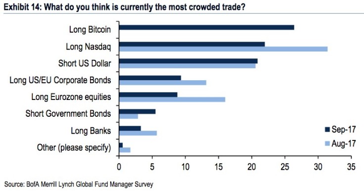
Bitcoin has been on a tremendous run and up almost 900% in 2017 alone. A recent institutional global survey asked respondents to identify the most crowded trade in the market: “Long Bitcoin” topped the list over “Long Nasdaq” and “Short USD”.  Recent events including the upcoming listing of Bitcoin futures by the CME and NASDAQ in early 2018 will open up the cryptocurrency market to even more investors.

 

Given that the word “bubble” has been used so frequently when describing Bitcoin, a Log-Periodic Power Law (LPPL) model is applied to see if it can accurately predict critical turning points in its exponential growth cycle.  LPPL models have their origins in statistical physics and are used to determine when a system is reaching a critical point.  While the original applications were in areas such as magnetism and  seismology,  the first use in economics was by Didier Sornette  in 1996, applying the search for critical points to the October 1987 market crash.  There have also been several studies on other financial assets including currency markets. (See Tranian 2012, Johansen 2013 ).

Financial markets are treated as a complex network of interacting traders. Under this theory, the aggregate behavior of all traders and investors can be modeled as a complex physical network.  As time progresses, the network of traders may become less idiosyncratic/individualistic and more correlated. Eventually, this network of traders transitions between the state of idiosyncratic behavior and  “herd” behavior.  In this state, external shocks can cause the entire system to “crash” and  “return to normal.” As the market self-organizes, oscillations occur and can be detected in the time series data. Measuring the strength of these oscillations through time allows one to quantify systemic risk.

While financial markets display exponential growth, they may not always display signs of periodic oscillations of increasing frequency. Just as in the rupture of a container under increasing pressure, these increasing periodic patterns only occur shortly before the rupture, or market crash.

Quick Theory Recap

The LPPL model is an oscillating, exponential model for price evolution. The intuition that underlies crash prediction is essentially the idea of the impossibility for continuing  exponential price growth, with increasing oscillations approaching failure indicated by swings in investor sentiment.

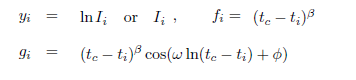
Mathematically, a basic LPPL model proposes that the price of an asset evolves at time t according to:

where:

ln[P(t)]  –  natural log of  Price p at time t
tc   –  the “Critical Time”  period i.e. the time of most probable crash
β (beta)  –  the exponential price growth with constraint   0 < β< 1
ω (omega) – the oscillation amplitude with general constraint   2 < ω < 20
ϕ (phi)  – a fixed phase constant parameter with constraint  0 < ϕ < 2π
A  – a constant equal to the log price at the Critical time (tc)  (ie. ln[P(tc)]  > 0 )
B(o) – a constant embodying the scale of power law where B(o) <0
C – a constant that captures the magnitude of the oscillation around price growth where|C| < 1

The conditions for β  and ω indicate “faster‐than-‐exponential” acceleration of the log‐price. The condition for ϕ expresses that the oscillations are neither too slow (such that they would simply become part of the trend) or too fast (such that they would fit the random component).

 

How to fit LPPL models?

The above equation has 7 parameters and 3 of the key ones (β, ω  and  ϕ ) are non-linear.  Therefore estimating LPPL models in general has never been easy due to the sheer number of parameters involved. However, rewriting and simplifying the LPPL equation as:

where

 

 

then we see that the linear parameters A, B, and C can be obtained by using ordinary least squares regression. Reducing the number of parameters from 7 to 4 helps simplify the calibration problem of the model.

The optimal values of the final 4 parameters (namely β, ω , ϕ and Tc) are found using a metaheuristic search algorithm such as Tabu search or a Genetic algorithm. However, a Simulated Annealing algorithmic approach was used here due to ease of implementation but the goal is the same, ie. using a probabilistic technique to approximate global optimization in a large search space. However, being metaheuristic, there is no guarantee of finding an optimum or near optimum solution of the cost function.

Data and Setup

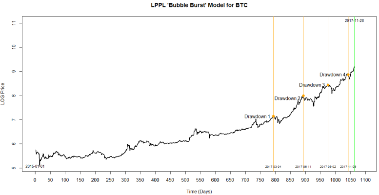
Historical aggregated daily trading data between 2015-1-1 to 2017-11-28 for Bitcoin USD price was used from Cryptocompare.com, giving a total of 1063 data points. To test the predictive power of the model, back testing was done on 4 key peaks in 2017 corresponding to drawdowns of at least 20% or more (shown in the table below). The LPPL model was then used to generate 30, 60 and 90 day forward estimates to examine the best time period window to predict near term crashes.

The drawdowns (orange lines) are shown below along with the current time period represented by the green line at time index 1063 (ie. 2017-11-28):

Example:
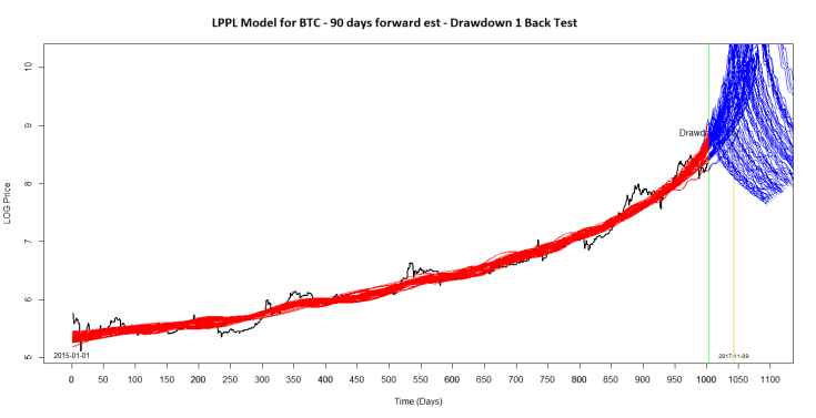
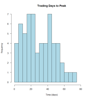
As an example: the plot below shows a back test simulation of a 90 day forward window for Drawdown 1 to see whether the median number of days from the green start line to Tc (Critical time for possible bubble burst) comes close to matching the actual date of the price crash (orange line).

The corresponding number of “Trading days to the peak” from the simulations can be summarized in a frequency plot below:

Along with a frequency plot for the “Peak price levels” obtained from the simulations :

As can be seen in this simulation for Drawdown 1, the median and mode estimates for the ‘number of days till the expected crash’ and the ‘expected peak price level’ at that time can be calculated.  In this particular simulation, the estimated median critical time (Tc) till crash was 45 days (~10 days early compared to the actual date) with a median equivalent peak price of $1085 (about ~14% below the actual peak price of $1267).

Backtest simulations were runs for 30D, 60D and 90D forward time estimates for all four drawdowns and the following results were generated:

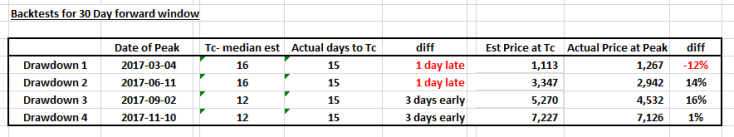
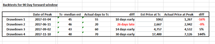
The results suggest that using a 60 day forward window would provide a relatively good balance between forecasting the Critical Time period (Tc) vs forecasting the expected Peak price at that time.

Results!

LPPL model using a 60 Day forward estimate :

The curve plot below corresponds to the optimal parameters found during the global metaheuristic algorithmic search.

Summary:

The top price plot shows that a near term Critical Time (tc) period is about 26 days from the last data point at 2017-11-28 (ie. 2017-12-24  X’mas Eve!).  The blue shaded zone on the plot corresponds to an 80% confidence interval for the predicted Critical Time.  The Peak Price equivalent in USD terms is a rather high ~$46,000 (vs current Bitcoin price of ~$11,000) and clearly assumes that Bitcoin’s exponential oscillating trajectory will continues at its current rapid rate. A more reasonable peak price assumption can be seen from the “Price Peak Level” Histogram which suggests a mode peak around the ~$25,000 range.

Caveats:
Models are always an approximation of reality! In particular the LPPL model has 7 parameters to estimate making precise calibration of the model tricky at best. Even though the simulation above suggests a ~70% pullback after hitting it’s price peak,  the LPPL model does not give an accurate forecast of how deep the “crash” will be when the bubble does burst.  Interestingly, other studies have shown that a “big crash” need not happen, as long as the price trend begins on a new longer sideways consolidation that effectively breaks away from the original accelerating exponential trend.

Disclaimer: This is not investment advice and is a practical example for illustrative purposes only. Please note that historical gains may not be representative of future returns. And as always before any investment, especially in cryptoworld, please thoroughly DYOR.  #DoYourOwnResearch

Happy Trading!
AJ